Clustering of municipalities

Introduction

In this part, we are going to take a closer look at our votations data and try to identify distinct communities (composed of the municipalities) with different votation patterns in Switzerland. In order to do so, we will use only the votation dataset and more specifically the results (in % Yes) of all the municipalities for all the votations since 1981 to nowadays as one single period of time (we are going to make the same exercise in a later post but analysing the data per decades). Thus, each municipality is represented by a vector of 312 components, each of them being the result (in % Yes) of a votation. The clustering methods used here are K-means and DBSCAN which will be quickly introduced below. Please note that the clustering is performed without dimension reduction as it is possible to run the algorithms in reasonable time. The PCA drawing the two first principal components are here to visualize the clustering, but the dimension reduction is performed after the clustering.

K-means

A quick introduction on K-means

K-means is a very popular clustering algorithm in data mining. It is an iterative refinement process with each iteration composed of two steps. At first, we chose arbitrarily or randomly either the initial cluster assignments or the initial clusters centers. We may also use more elaborated initialization algorithms such as kmeans++ which is the default initialization in sklearn (the library we use). However, we will not detail those methods here. Then, each iteration performs the following steps:

• Assignment step: each observation is assigned to the cluster center which is the closest to it (the distance being computed as the squared Euclidean distance).
• Update step: the clusters centers are updated as the mean of the points belonging to the cluster.

The iterative processes may stop and the final assignment reached for two reasons. First, the clusters may no longer change, i.e., the observations stayed assigned to the same centers in the assignment step and we say that the algorithm converged. Secondly, the maximal number of iteration may be reached. This second condition is sometimes necessary as the convergence is not guaranteed.

A disadvantage of K-means is the shape of the clusters which are hyper-spherical (circles in 2D, spherical in 3D, etc.) due to the Euclidean distance. This limitation may be an issue if the underlying data have natural categories which are not shaped as hyper-spheres. Another limitation is the fact that the number of clusters K has to be chosen before running the algorithm. This means that the number of clusters has to be chosen carefully not to create categories which have no interpretation. Also, K-means forces all the points to belong to a cluster. This behavior may be desirable to avoid points which are not clustered, but make the cluster less meaningful if the outliers are numerous. Note that these limitations are not present in DBSCAN.

Maps (results)

K-means, k=2 k-means, k=3 k-means, k=4 k-means, k=5

See the full map here

Analysis and discussion

It is very important to note that K-means has essentially only one parameter which is the number of clusters. Thus, it is nearly impossible to influence it in order to show a specific a result. What may influence the final clusters in the iterative process of K-mean is the initial centers positions of the clusters and the number of iterations. In our case, we let sklearn deals with its default values. Thus, the algorithm is run 10 times with different initial clusters centers chosen randomly with a maximum of 300 iterations if the convergence is not reached with fewer. The final result is the best classification of the 10 consecutive runs in terms of inertia, i.e., minimizing the within-cluster sum of squared. It must be said that the results are not influenced anyhow by us.

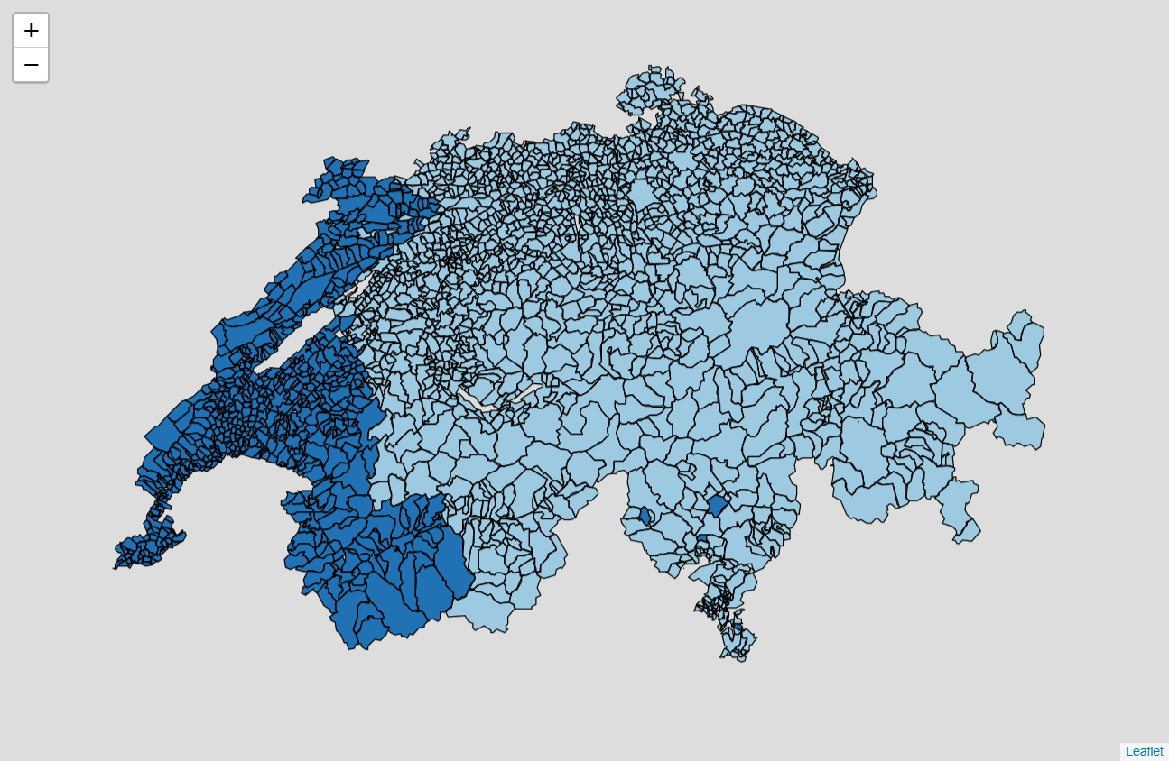
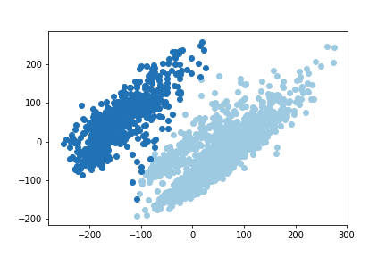
Two clusters

When we try to classify our votation data into two categories, it is clear that two distinct communities appear. On one side the Romandy (French community) and on the other side the rest of Switzerland (German, Italian and Romansh communities). A reader may quickly take a look at our map of the languages spoken in Switzerland drawn in previous post. Looking at the visualization of the two first principal components of the PCA, we can see that the two categories are distinguishable by human eyes and the algorithm correctly classified them. Thus, we successfully identify a Röstigraben pattern in our data.

This result is very strong and lets quickly explain why. The K-mean algorithm here is does not use any geographical or linguistic features, i.e., the algorithm is unaware of the geographical position of a municipality or the language spoken there. Yet, except few municipalities in Ticino classified with Romandy and few municipalities in Berner Jura (Romandy region which is attached to the canton of Bern) classified with the German region, the algorithm categorized the municipalities into two geographical/linguistic categories corresponding to the exact linguistic frontier between the French and the German communities in Switzerland. The existence of differences in votations patterns between French speaking and German speaking citizens is undeniable.

Three clusters

As the French community stays united, we see that the second category while we were considering two clusters is now split. The new category represents the urban area of the German community (Zurich, Bern, St. Gallen, Thun and Basel) together with Ticino and Grisons. This results let suggests that the urban areas in the German community have a different voting pattern than the countryside. A result which will be validated later when we will cluster the votations by decades. Moreover, the demarcation of Ticino begins to be perceived but it not yet strong enough to separate it from the rest of the German community. The PCA does not show a strong split between the second and the third category, but it has to be noted that the clustering is performed without dimension reduction and the PCA drawn takes the data from 312 dimensions down to 2 dimensions. Even if those dimensions are the principal components, it hides the information of the 300 other dimensions.

Four clusters

Now, while the previously identified categories stay the same, Ticino represents the new category. This is also referred as the Polentagraben, i.e., Ticino has different voting patterns than the rest of Switzerland. However, we can note that as this pattern border has not been identified earlier while we considered two and three clusters, the result is weaker than the Röstigraben and the urban-countryside split in the German community. Nonetheless, it does exist.

Again, we can note that the way we used K-means the algorithm is not aware of any geographical or linguistic features. Thus, Ticino just as the Romandy represents one cluster only because they have different voting patterns compare to the other identified clusters.

Five clusters

Again, the previously identified clusters remain unchanged except for the Romandy now represented over two categories. The first one is led by Geneva and Vaud. The second is composed of Valais, Fribourg, Jura, the Berner Jura and Upper Neuchâtel.

DBSCAN

A quick introduction on DBSCAN

DBSCAN (Density-Based Spatial Clustering of Applications with Noise) is another clustering algorithm. The algorithm takes only two parameters, i.e., the distance (ε) and the minimum number of points which has to stand within a radius ε to be considered as a cluster. The algorithm starts with a point and check its neighborhood in the radius ε, if it contains at least the minimum number of points given as parameter a new cluster is created. Then, each points of the neighborhood are walked to find other points at a maximum distance of ε which will be added to the cluster. When it is not possible to add more points, the cluster reached its final shape. Non-clustered points are then visited to create new clusters based on the same criteria than previously. Points may not be classified in a cluster if they are not in the neighborhood of existing clusters or if there are not enough points to create a new cluster in their own neighborhood. Such points are called outliers (or noise).

The advantage of DBSCAN over K-means is that it does not require the number of clusters to be given as parameter and it is able to handle clusters of arbitrary shape. Also, DBSCAN is able to deal with data cointaining noise making clusters more meaningful, but letting points unclustered.

The main disadvantage of DBSCAN is that we have to choose its parameters carefully. Basically, the parameters represent the estimated density of the clusters to be considered which is dependent on the data. On one hand, if the density is overestimated the cluster will not be propagated. On the other hand, if the density is underestimated the noise will be clustered. Practically, one can try multiple values for the parameters until the results looks visually correct (which we partially did, see below).

Maps (results)

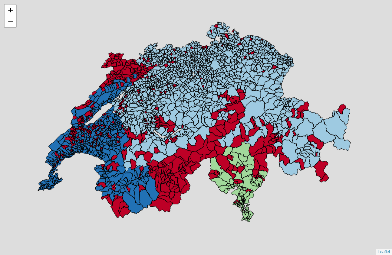
For the result we present below, we took a minimum number of points of 20 which is intentionally low as we deal with a lot of outliers. For the distance, we computed the average distance of the 39 closest neighbors of each observation and we took the average of these values. On the map, the outliers are drawn in dark red and the clusters are represented by the other colors.

See the full map here

Analysis and discussion

Our DBSCAN identified three clusters. The first one represents Romandy (Vaud, Geneva, Neuchâtel, French speaking Fribourg, French speaking Valais and the Berner Jura). The second cluster represents the canton of Ticino and the third the German speaking Switzerland. Important outliers’ regions are Jura, the German speaking Valais and the Italian speaking Grisons.

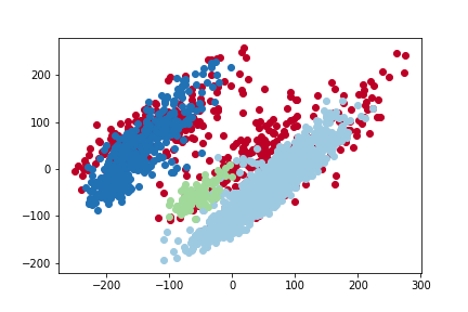
This result confirms what we previously obtained with K-means. It shows different voting patterns in Romandy (Röstigraben) and in Ticino (Polentagraben). The results are now a little bit mitigated as now the outliers are not classified anymore. However, the clusters themselves are stronger. The PCA shows that we obtained a clustering which is meaningful as the clusters are distinguishable by human eyes.

Just as for K-means it has to be noted that the DBSCAN algorithm is not aware of the linguistic regions or the geographical structure of the country (which municipalities are physically neighbors). This again makes the results stronger has we found distinctive linguistic/geographical patterns in similar voting behaviors. It also has to be said that nothing prevents a municipality geographically in a cluster to belongs to another cluster (as the geographical structure is not a feature). However, it never happens. If a municipality is geographically inclusive in a cluster but does not belong to it, then it has been categorized as an outlier. This remark also gives more credit to the geographical patterns identified.

Conclusion

Through this post we identified regions in Switzerland with similar voting behavior. The results are strong and show that the Romandy and Ticino tends to vote differently compare to the rest of Switzerland, mainly the German speaking Switzerland. This difference in cultural behavior is commonly referred as Röstigraben and Polentagraben and we showed that it is not only sayings between elders, but behavior that is reflected in the votations since 1981.

Our results are meaningful as the algorithm and the data we used make a total abstraction of underlying geographical or linguistic features in the country. Yet, we can identify them clearly using only the votation data.

To go further in our analysis, we may consider to process old and recent votations in order to see if this behavior is changing over time. It is also possible that our results have been influenced by strong components in specific timeframe which would make the results not representative of more recent voting patterns. This is the subject of a further post.